If your dataset is starting to get big or uses loosely related information, keeping a master sheet that links to all others allows you to get a clear overview and pass on vital information. Rather than copying verbatim, a master sheet allows you to use links to automatically update data. Here’s how to make a link to a master sheet in Excel and keep your sheets organized.
Contents
Option 1 – Link to a Master Sheet Using a Basic Cell Reference
The simplest way to pull data from or to a master sheet is a direct cell reference. This works for any single value that needs to be passed between sheets.
Step 1. Click on the cell in the sheet where you want the linked value to appear.
Step 2. Type an equals sign (=) to begin the formula, then click on the tab for your target sheet at the bottom of the workbook. The formula bar will show the sheet name followed by an exclamation mark automatically.
Step 3. Click the cell you want to pull from and hit “Enter.” Excel will return you to the original sheet with the linked value now displaying.
Alternatively, you can type the reference directly without clicking. The syntax is =SheetName!CellAddress, so to pull cell B2 from a sheet named “Revenue,” you would type =Revenue!B2. If the sheet name contains spaces (for example, “Revenue 2026”), wrap it in single quotes: =‘Revenue 2026’!B2.
Option 2 – How to Link Sheets in Excel to a Master Sheet as a List
If you want the master sheet to contain the links to the respective sheets (perhaps to a particular cell), you can use the HYPERLINK function with the syntax:
HYPERLINK (link_location, [friendly_name])
The link location here is tricky, as it needs to be parsed from a series of characters and in the format of “#SheetName!Cell.” The “friendly name” part is just how the hyperlink will look (its name).
To do that, you’ll need to use the following formula for the link location: “#’”&CellReference&”‘!Cell” where:
- CellReference is the name of the sheet as listed in the master sheet and in Excel (the names must match.
- Cell is the target cell of the sheet you’re linking to, such as A1, C3, and so on.
For example, suppose we have a simple master sheet of yearly revenues.

Step 1. If you want to put links for each sheet, you can use the formula for the first option as: =HYPERLINK(“#'”&B2&”‘!A1”, B2)
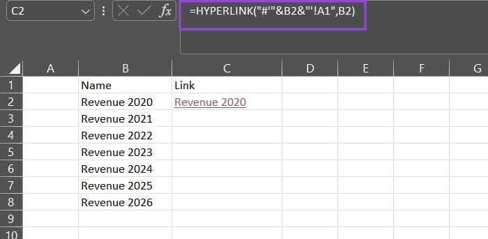
Excel will fetch the name listed in B2 (in this case “Revenue 2020”) and make a link to the sheet “Revenue 2020” to its cell A1. The “friendly name” is simply copied for simplicity.
Step 2. Flash fill or drag the fill handle down to apply the formula, and Excel will automatically iterate through the cell range.
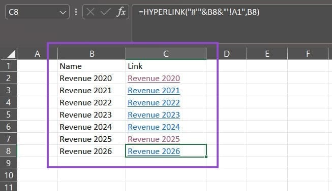
Step 3. If you want to add a new sheet to the master sheet, just add a new row to the bottom and replicate the formula. Make sure its name is exactly as listed in the Sheet toolbar at the bottom.
Note that the links don’t have to be sequential (as ordered in Excel).
Option 3 – Use Named Ranges to Link Cells to a Master Sheet
Instead of referencing specific cell addresses, you can give a cell a “name” that it will be known as throughout the process.
Step 1. Select the cell or range you want to name.
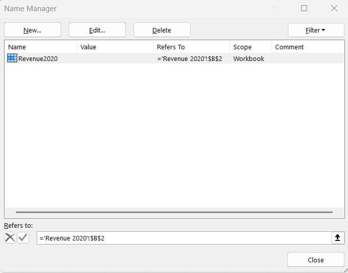
Step 2. Click in the Name Box in the top-left corner of the screen, just above column A. Type in a descriptive name and hit “Enter” to confirm. For example, we’ve named the cell B2 of the sheet “Revenue 2020” as “Revenue2020.”
You can use the “Name Manager” to look at the current list of names.
Note that you can’t make the name “ABC123” (three letters then numbers), as that is an acceptable cell reference for an Excel table.
Step 3. On any other sheet in the workbook, you can now reference that value simply by typing “=Name” (without the quotes). You will also get the name as a suggestion when typing in formulas.
Step 3b. If you want to pass on a link to the cell rather than the value, use the formula: =HYPERLINK(“#Name”,link_name)

Step 4. If you made the name ranges follow a pattern, you can emulate that pattern by having the master sheet create hyperlinks to respective sheets.
Suppose each named range follows a naming convention of “RevenueXXXX” where “XXXX” is the year.
You can then put the years in column B and the following formula in the respective cells in C:
=HYPERLINK(“#”&CELL(“address”,INDIRECT(“Revenue”&B2)),”Revenue “&B2)
This passes the “Revenue” part of the name manually, then the cell reference from the year range.