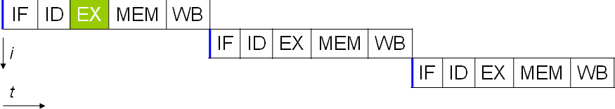
Early computers were entirely sequential. Each instruction the processor received needed to be completed in full in order before the next one could be started. There are five stages to most instructions: Instruction fetch, Instruction decode, Execute, Memory access, and Writeback. Respectively these stages get the instruction that needs to be completed, separate the operation from the values being operated on, execute the operation, open the register on which the result will be written, and write the result to the opened register.
Each of these stages should take one cycle to complete. Unfortunately, if the data isn’t in a register, then it must be requested from the CPU cache or the system RAM. This is a lot slower, adding dozens or hundreds of clock cycles of latency. In the meantime, everything else needs to wait as no other data or instructions can be processed. This type of processor design is called subscalar as it runs less than one instruction per clock cycle.
Pipelining to scalar
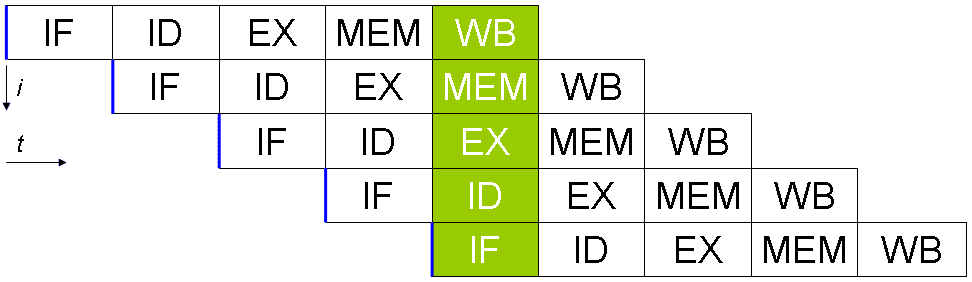
A scalar processor can be achieved by applying a system pipeline. Each of the five stages of an instruction being executed run in different bits of hardware in the actual processor core. Thus, if you’re careful with the data you feed into the hardware for each stage, you can keep each of them busy every cycle. In a perfect world, this could lead to a 5x speed up and for the processor to be perfectly scalar, running a full instruction per cycle.
In reality, programs are complex and reduce the throughput. For example, if you have two addition instructions “a = b + c” and “d = e + f” these can be run in a pipeline with no issue. If, however, you have “a = b + c” followed by “d = a + e” you have a problem. Assuming these two instructions are directly after one another, the process to calculate the new value of “a” won’t have completed, let alone be written back to memory before the second instruction reads the old value of “a” and then gives the wrong answer for “d”.
This behaviour can be countered with the inclusion of a dispatcher, that analyses upcoming instructions and ensures that no instruction that is dependent on another is run in too close succession. It actually runs the program in the wrong order to fix this. This works, because many instructions don’t necessarily rely on the result of a previous one.
Expanding the pipeline to superscalar
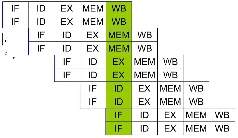
A superscalar processor is capable of running more than one full instruction per cycle. One way of doing this is by expanding the pipeline so that there are two or more bits of hardware that can handle each stage. This way two instructions can be in each stage of the pipeline in every cycle. This obviously results in increased design complexity as hardware is duplicated, however, it offers excellent performance scaling possibilities.
The performance increase from increasing pipelines only scales so far efficiently though. Thermal and size constraints place some limits. There are also significant scheduling complications. An efficient dispatcher is now even more critical as it has to ensure that neither of two sets of instructions relies on the result of any of the other instructions being processed.
A branch predictor is a portion of the dispatcher that gets more and more critical the more highly superscalar a processor is. Some instructions can have two potential outcomes, each one leading to different following instructions. A simple example would be an “if” statement. “If this is true do that, otherwise do this other thing”. A branch predictor attempts to predict the outcome of a branching operation. It then pre-emptively schedules and executes the instructions following what it believes to be the likely outcome.
There is a lot of complex logic in modern branch predictors, that can result in branch prediction success rates on the order of 98%. A correct prediction saves the time that could have been wasted waiting for the actual result, an incorrect prediction necessitates that the predicted instructions and any of their results be discarded and the true instructions be run in their place, which comes with a slight penalty over having just waited. Thus high-prediction success rates can increase performance noticeably.
Conclusion
A computer processor is considered superscalar if it can perform more than one instruction per clock cycle. Early computers were entirely sequential, running only one instruction at a time. This meant that each instruction took more than one cycle to do complete and so these processors were subscalar. A basic pipeline that enables the utilisation of the stage-specific hardware for each stage of an instruction can execute at most one instruction per clock cycle, making it scalar.
It should be noted that no individual instruction is fully processed in a single clock cycle. It still takes at least five cycles. Multiple instructions, however, can be in the pipeline at once. This allows a throughput of one or more completed instructions per cycle.
Superscalar should not be confused with hyperscaler which refers to companies that can offer hyperscale computing resources. Hyperscale computing includes the ability to seamlessly scale hardware resources, such as compute, memory, network bandwidth, and storage, with demand. This is typically found in large data centres and cloud computing environments.